 Cameron MacLeod
abracadabra: How does Shazam work?
Sat 19 February 2022 Tutorials
Your phone's ability to identify any song it listens to is pure technological magic. In this article, I'll show you how one of the most popular apps, Shazam, does it. The founders of Shazam released a paper in 2003 documenting how it works, and I have been working on an implementation of that paper, abracadabra.
Where the paper doesn't explain something, I will fill in the gaps with how abracadabra approaches it. I've also included links to the corresponding part of the abracadabra codebase in relevant sections so you can follow along in Python if you prefer.
The state of the art has moved on since this paper, and Shazam has probably evolved its algorithm. However, the core principles of audio identification systems haven't changed, and the accuracy you can obtain using the original Shazam method is impressive.
To get the most out of this article, you should understand:
Quick links
What is Shazam?#
Shazam is an app that identifies songs that are playing around you. You open the app while music is playing, and Shazam will record a few seconds of audio which it uses to search its database. Once it identifies the song that's playing, it will display the result on screen.
Before Shazam was an app, it was a phone number. To identify a song, you would ring up the number and hold your phone's microphone to the music. After 30 seconds, Shazam would hang up and then text you details on the song you were listening to. If you were using a mobile phone back in 2002, you'll understand that the quality of phone calls back then made this a challenging task!
Why is song recognition hard anyway?#
If you haven't done much signal processing before, it may not be obvious why this is a difficult problem to solve. To help give you an idea, take a look at the following audio:
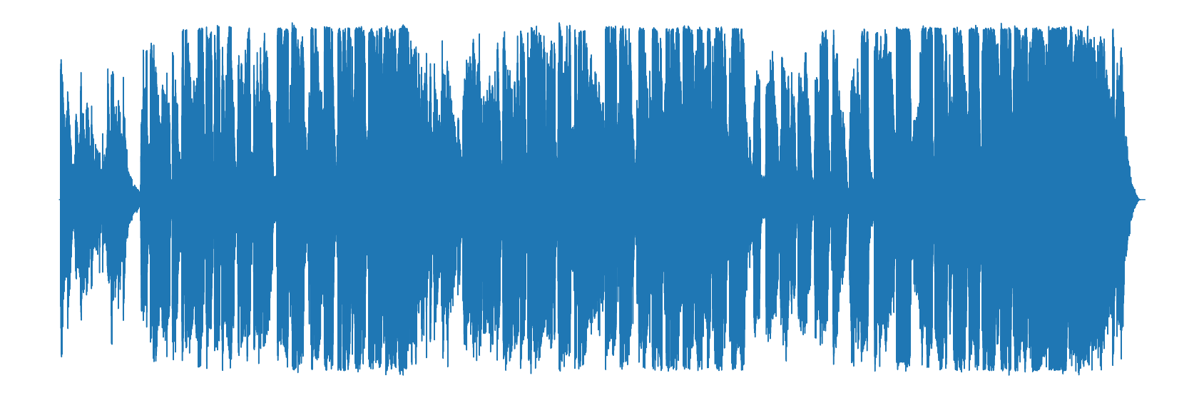
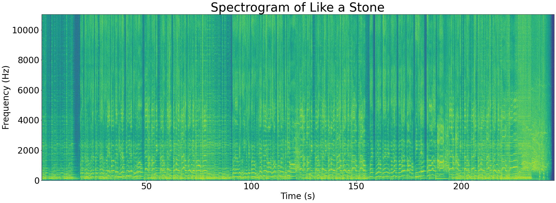
The above graph shows what Chris Cornell's "Like a Stone" looks like when stored in a computer. Now take a look at the following section of the track:
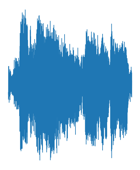
If you wanted to tell whether this section of audio came from the track above, you could use a brute-force method. For example, you could slide the section of audio along the track and see if it matches at any point:
This would be a bit slow, but it would work. Now imagine that you didn't know which track this audio came from, and you had a database of 10 million songs to search. This would take a lot longer!
What's worse, when you move from this toy example to samples that are recorded through a microphone you introduce background noise, frequency effects, amplitude changes and more. All of these can change the shape of the audio significantly. The sliding method just doesn't work that well for this problem.
Thankfully, Shazam's approach is a lot smarter than that. In the next section, you'll see the high-level overview of how this works.
System overview#
If Shazam doesn't take the sliding approach we described above, what does it do? Take a look at the following high-level diagram:
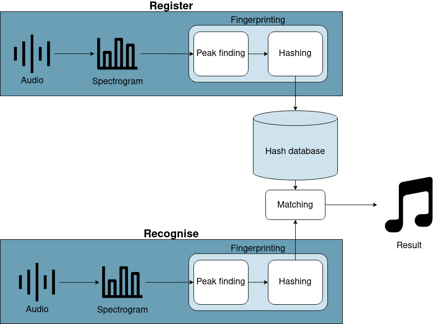
The first thing you will notice is that the diagram is split up into register and recognise flows. The register flow remembers a song to enable it to be recognised in the future. The recognise flow identifies a short section of audio.
Registering a song and identifying some audio share a lot of commonality. The following sections will go into more detail, but both flows have the following steps:
- Calculate the spectrogram of the song/audio. This is a graph of frequency against time. We'll talk more about spectrograms later.
- Find peaks in that spectrogram. These represent the loudest frequencies in the audio and will help us build a fingerprint.
- Hash these peaks. In short, this means pairing peaks up to make a better fingerprint.
After calculating these hashes, the register flow will store them in the database. The recognise flow will compare them to hashes already in the database to identify which song is playing through the matching step.
In the next few sections, you'll learn more about each of these steps.
Calculating a spectrogram#
The first step for both flows is to obtain a spectrogram of the audio being registered or recognised. To understand spectrograms, you first have to understand Fourier transforms.
The Fourier transform#
A Fourier transform takes some audio and tells you which frequencies are present in that audio. For example, if you took a 20 Hertz sine wave and used the Fourier transform on it, you would see a big spike around 20 Hertz (Hz):
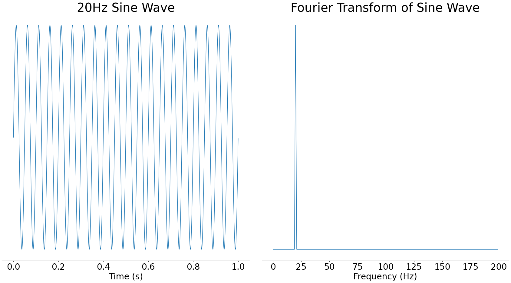
In the above image, you can see a large spike around 20Hz and nothing at other frequencies. Sine waves are often called pure tones because of this property, since they only contain a single frequency.
The result of a Fourier transform is called a frequency spectrum. We say that when you take the Fourier transform of a signal, you move it from the time domain into the frequency domain. These are fancy terms for describing whether time or frequency is along the bottom of a graph. In mathematical terms, the domain is more or less the X-axis of a graph.
The Y-axis of the frequency spectrum represents the strength of each frequency component. If a frequency component is stronger, then it will be more audible in the time-domain signal.
If you were to add a 50Hz sine wave at half the strength to that 20Hz sine wave, the resulting frequency spectrum would show a spike at 20Hz and a smaller spike at 50Hz:
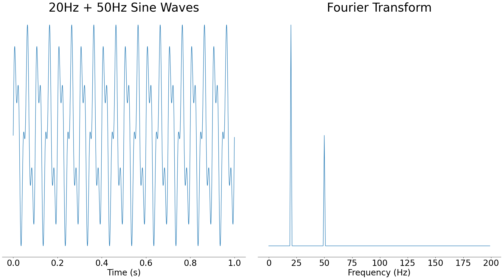
As you can see, adding multiple audio waves together combines the frequencies present in them. In fact, all audio signals can be reconstructed from waves like this. For more, take a look at 3Blue1Brown's video on the Fourier transform.
One great property of the frequency domain is that it often helps us to see things that aren't clear in the time domain. For example, if you take the signal with two frequencies from before and add noise to it, in the time domain it looks visually very different. However, in the frequency domain, the two spikes are still very clear:
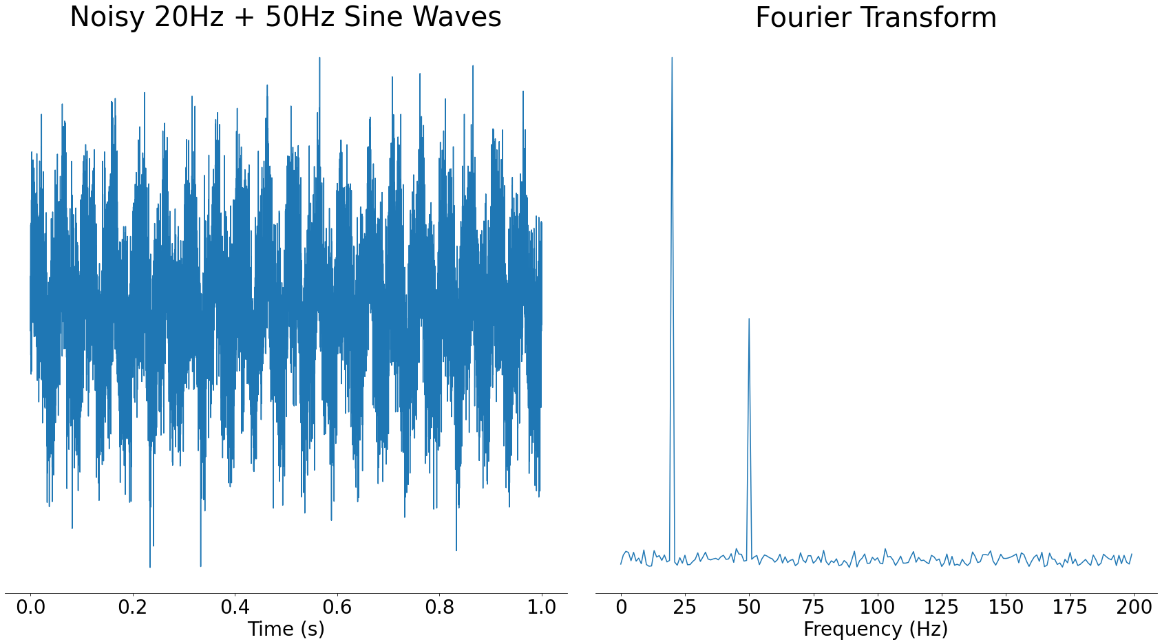
In the frequency domain graph on the right, you can still clearly see the spikes for the main component frequencies. It would be harder in the time domain to see what frequency sine waves went into the signal.
Up until now, our examples have only contained one or two frequencies, but what happens if you put a more complex signal through the Fourier transform? Let's take a look at our section of audio from Like a Stone:
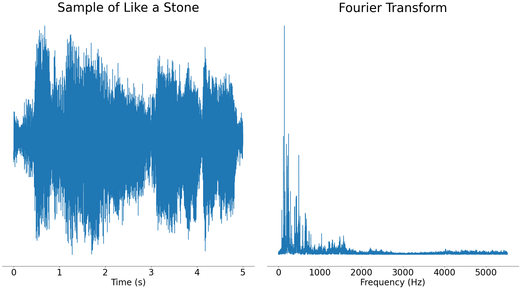
Real audio files like the one above contain lots of different frequencies. This is a good thing, as it means that the frequencies present can uniquely identify songs.
Spectrograms#
If you run a Fourier transform over an entire song, then you will see the strength of the frequencies present over the whole song. However, the frequencies that are present change over time. To better represent the frequencies changing over time, we need to split the song into small sections before taking the Fourier transform. This is called taking a spectrogram.
Here's a simplified animation of how spectrograms work:
In the above animation, you can see that the song is first split into small sections. Next, we use the Fourier transform to calculate the frequency spectrum of each of these sections. When you put all these frequency spectrums together, you get a spectrogram.
To make this concrete, let's take a look at the spectrogram of Like a Stone:
Even though the spectrogram looks 2-dimensional, it's actually a 3D graph with the following axes:
- Time (X-axis)
- Frequency (Y-axis)
- Strength (Z-axis/colour)
The Z-axis is represented by colour in the spectrogram above. Bright green shows a high magnitude for a particular frequency component and dark blue shows a low magnitude.
Looking at the spectrogram above, you can see that the brightest spots (strongest frequencies) almost exclusively occur below 5000Hz. This is quite common with music, for example most pianos have a frequency range of 27Hz-4186Hz.
The frequencies present in a track contain a lot of identifying information, and calculating the spectrogram allows us access to that information. In the next section, you'll learn how we turn all that information into a unique fingerprint for the track.
Fingerprinting#
Just as a fingerprint uniquely identifies a person, we can extract a unique fingerprint for some audio from its spectrogram.
These audio fingerprints rely on finding peaks in the spectrogram. These peaks are the loudest frequencies at some time in the song. Because they are loud, it's likely they'll survive when subjected to noise or other distortions.
In the next section, you'll read some more about the motivation behind using spectrogram peaks to build fingerprints.
Why is the fingerprint based on spectrogram peaks?#
A spectrogram peak is a frequency that is loud at some point in an audio signal. You can recognise these on a spectrogram since they will be the brightest points.
In music, these would represent the loudest notes. For example, during a guitar solo, the notes that the guitar is playing might become spectrogram peaks since they would likely be the loudest notes at that time.
A spectrogram peak is the point least likely to be affected by noise. Noise has to be louder than the spectrogram peak to make it unrecognisable and the spectrogram peaks are the loudest frequency components in the track.
To make this visual, take a look at our earlier example of a Fourier transformed signal that had noise added to it. When noise is added, the frequency peaks still retain their rough shape.
Another advantage of using spectrogram peaks to fingerprint audio is that they cut down the amount of data we have to store. Storing only the loudest frequency components means we don't have to store everything else. This speeds up searching fingerprints since there is less data to look through.
Before we can use frequency peaks in our fingerprint though, we have to find them. In the next section, you'll learn how.
Finding peaks#
As discussed in the previous section, the peaks of a spectrogram represent the strongest frequencies in a signal. For frequency peaks to be usable in an audio fingerprint, it's important that they are evenly spaced through the spectrogram.
It's important the peaks are evenly spaced in time, so the system can recognise any section of the song. For example, if all the peaks were at the start of the song, then the fingerprint wouldn't cover later sections:
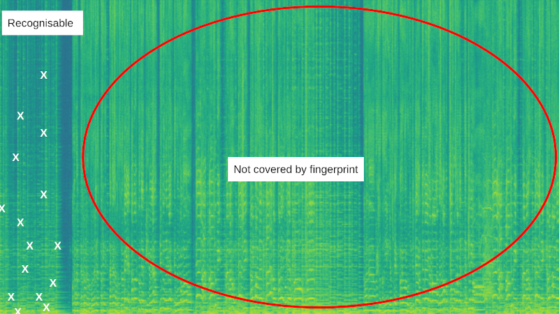
In the image above, all the peaks (white crosses) are clustered at the start of the song. This means that the system can't recognise any sample from the rest of the song.
It's also important that the peaks are evenly spaced in frequency, so the system can deal with noise and frequency distortion. Sometimes noise will be very loud and concentrated at a specific frequency range, for example a car horn in the background:
In the above animation, the peaks are well-spaced in time, but are clustered into a small frequency band. When a loud noise is introduced, for example a car horn, it can make an entire section of song unrecognisable by changing which peaks are selected.
To find spectrogram peaks while keeping them well-spaced, we can borrow a technique from image processing known as a maximum filter. The process looks something like the following:
- Use the maximum filter to highlight peaks in the spectrogram.
- Locate the highlighted peaks by comparing to our original spectrogram.
- (Optional) Discard some peaks.
Let's run through these steps one-by-one. First, let's take a look at how the maximum filter works:
Step 1: Maximum filter
A maximum filter emphasises the peaks in an image. It does this by looking in a neighbourhood around each pixel for the maximum value and then setting the pixel to that local maximum. The following animation shows a maximum filter that looks at a 3x3 neighbourhood around each pixel:
As you can see in the above animation, the maximum filter takes each pixel of an image in turn and finds the maximum in a region surrounding it. The filtered pixel is then set to that local maximum. This has the effect of expanding each local peak to its surrounding area.
Running a maximum filter on Like a Stone's spectrogram gives the following result:
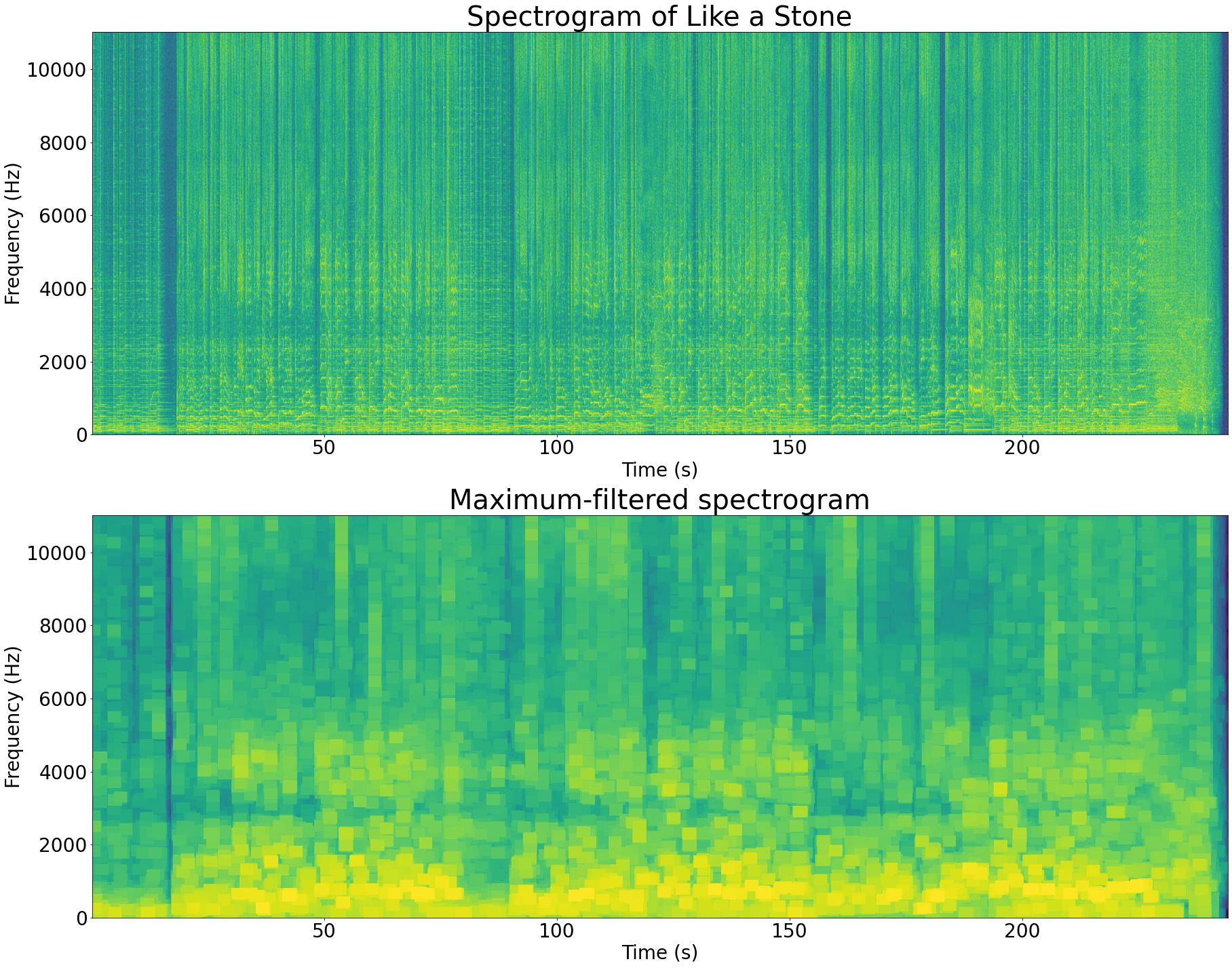
The maximum-filtered spectrogram looks like a lower-resolution version of the original spectrogram. This is because the peaks in the signal have expanded and taken over the other pixels. Each box with the same colour in the filtered image corresponds to a local peak in the original image.
The maximum filter has a parameter that controls the size of the box to use when finding the local maxima. When you set this parameter to make a smaller box, you end up getting more peaks. Similarly, by setting this parameter larger you get fewer peaks.
Step 2: Recover original peaks
The maximum filter doesn't do all the work for us. The filter has emphasised the local peaks, but it hasn't found their locations. To find the peak locations, we need to find the points that have equal values in the original spectrogram and the filtered spectrogram.
The idea behind this trick is that all the non-peak points in the spectrogram have been replaced by their local peaks, so their values have changed. The only points whose values haven't changed are the peaks.
Below is a zoomed in section of the spectrogram above. The points where the values are equal in the filtered and original spectrograms are highlighted:
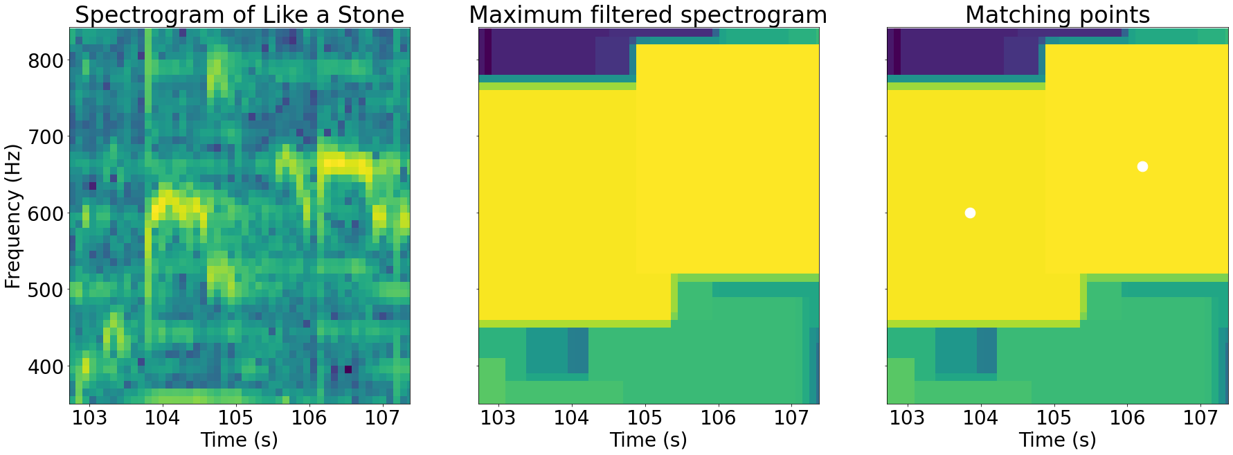
As you can see in the images above, the highlighted points where the two spectrograms are equal correspond to the local peaks of that part of the image.
Plotting all of the peaks together produces something called a constellation map. Here's the constellation map for Like a Stone:
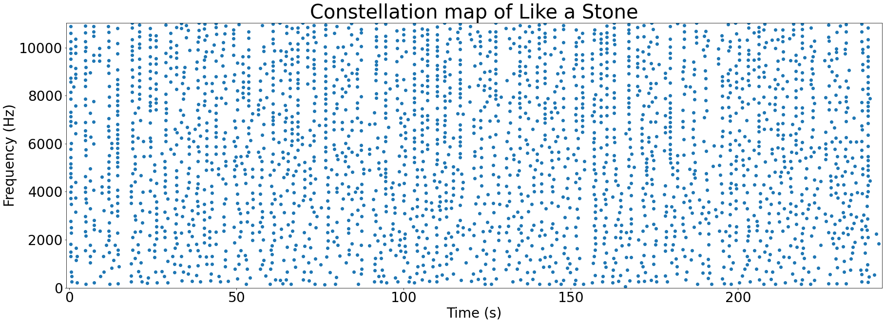
These graphs are called constellation maps since they look a bit like an image of the night sky. Who said computer science couldn't be romantic?
Step 3: (Optional) Discard peaks
Once we have a constellation map of peaks, the next step is to potentially discard some. The size of our fingerprint is dependent on the number of peaks that we use in it. Keeping fingerprints small matters when you are storing millions of songs in your database.
However, by reducing the number of peaks we use, we reduce the accuracy of our system. Fewer peaks in a fingerprint mean fewer chances to match a sample to the correct song.
There are a couple of options for reducing the number of peaks in our fingerprint:
- Take the top N peaks. N should be proportional to the length of audio that you are fingerprinting to avoid over-representing shorter songs.
- Take all peaks above a certain threshold. This doesn't guarantee you a certain fingerprint size per time like the other method, but may give more accurate results.
We have almost finished constructing our fingerprint, the next step is to produce a set of hashes from our peaks.
Hashing#
To motivate hashing, imagine that our fingerprint was just a collection of spectrogram peaks. Each peak's frequency would be represented by a certain number of bits, for example 10. With 10 bits of information, we can represent 2^10=1024 individual frequencies. With thousands of these points per track, we quickly get a lot of repeats.
Uniqueness is important for a fingerprint, since it makes searching a lot faster and helps to recognise more songs. Shazam's solution to the problem of uniqueness is to create hashes from pairs of peaks:
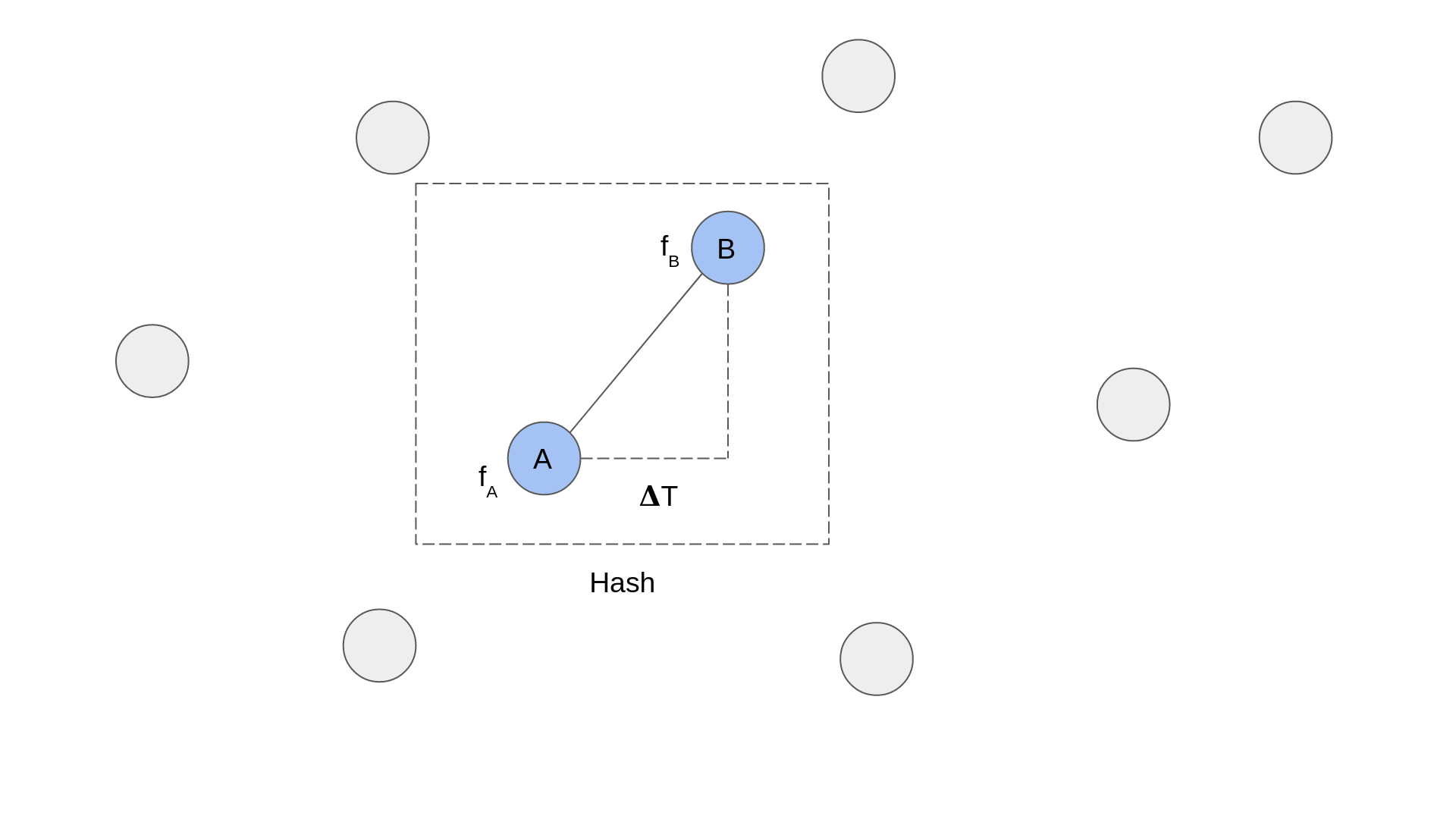
The diagram above shows a zoomed in portion of a spectrogram. Each circle represents a peak and the dashed line box represents a hash. You can see that a hash is formed of two peaks. The information that is recorded for each hash is the frequency of each peak, fA and fB, and the time delta between them, 𝚫T.
The advantage of pairing points up is that two paired points are much more unique than a single point. Looking at it mathematically, if each point has 10 bits of frequency information, and the time delta between the two points could be represented by 10 bits, then you have 30 bits of information. 2^30=1073741824 which is significantly larger than 1024 possibilities for a single point.
Shazam creates pairs using the following algorithm:
- Pick a point. This will be called the anchor point.
- Calculate a target zone of the spectrogram for the anchor point.
- For every point in the target zone, create a pair with the anchor point.
You can see this algorithm illustrated in the following animation:
Choosing a target zone isn't described in the Shazam paper, but the images the paper contains show it as starting slightly ahead of time of the anchor point and being centred on the anchor point's frequency.
Once a pair has been created, it is stored as a hash in the database with the following information:
| Other information | ||||
|---|---|---|---|---|
| Point A freq (fA) | Point B freq (fB) | Time delta (𝚫T) | Point A time | Track ID |
The first three columns (fA, fB and 𝚫T) make up the hash. The "Other information" is used to locate the hash at a specific time in a song. This will be used in matching later.
All of the hashes for a particular track make up the fingerprint. In the next section, you'll read about how Shazam matches these fingerprints.
Matching#
Given a collection of fingerprints in a database, how does Shazam figure out which one a given audio sample matches? This is where the matching part of the system comes in. Recall the system diagram from earlier:
The recognise and register flows both generate fingerprints. The difference lies in what they do with them. While the register flow stores fingerprints away for future matching, the recognise flow has to match its fingerprint with what is already in the database.
The matching algorithm contains the following steps:
- Retrieve all hashes from the database that match the sample's fingerprint.
- Group these hashes by song.
- For each song, figure out if the hashes line up.
- Choose the track with the most lined up hashes.
We'll look at each of these steps in turn.
Step 1: Retrieve matching hashes
The first step is to find every hash in the database that matches a hash in the fingerprint we just created. Even though a hash is a 3-tuple of (fA, fB, 𝚫T), abracadabra stores this as hash(fA, fB, 𝚫T) where hash() is a hash function that returns a single value. This way you only have to search for a single value per hash instead of three.
Step 2: Group hashes by song
Recall the format of an individual hash in the database:
| Other information | ||||
|---|---|---|---|---|
| Point A freq (fA) | Point B freq (fB) | Time delta (𝚫T) | Point A time | Track ID |
Thanks to the track ID that we associated with each hash, we can group the hashes by track. This allows us to score each potentially matching track.
Step 3: Figure out if hashes line up
If a sample matches a song, then the hashes present in that sample should line up nicely with the hashes in some section of that song. The diagram below illustrates what this would look like:
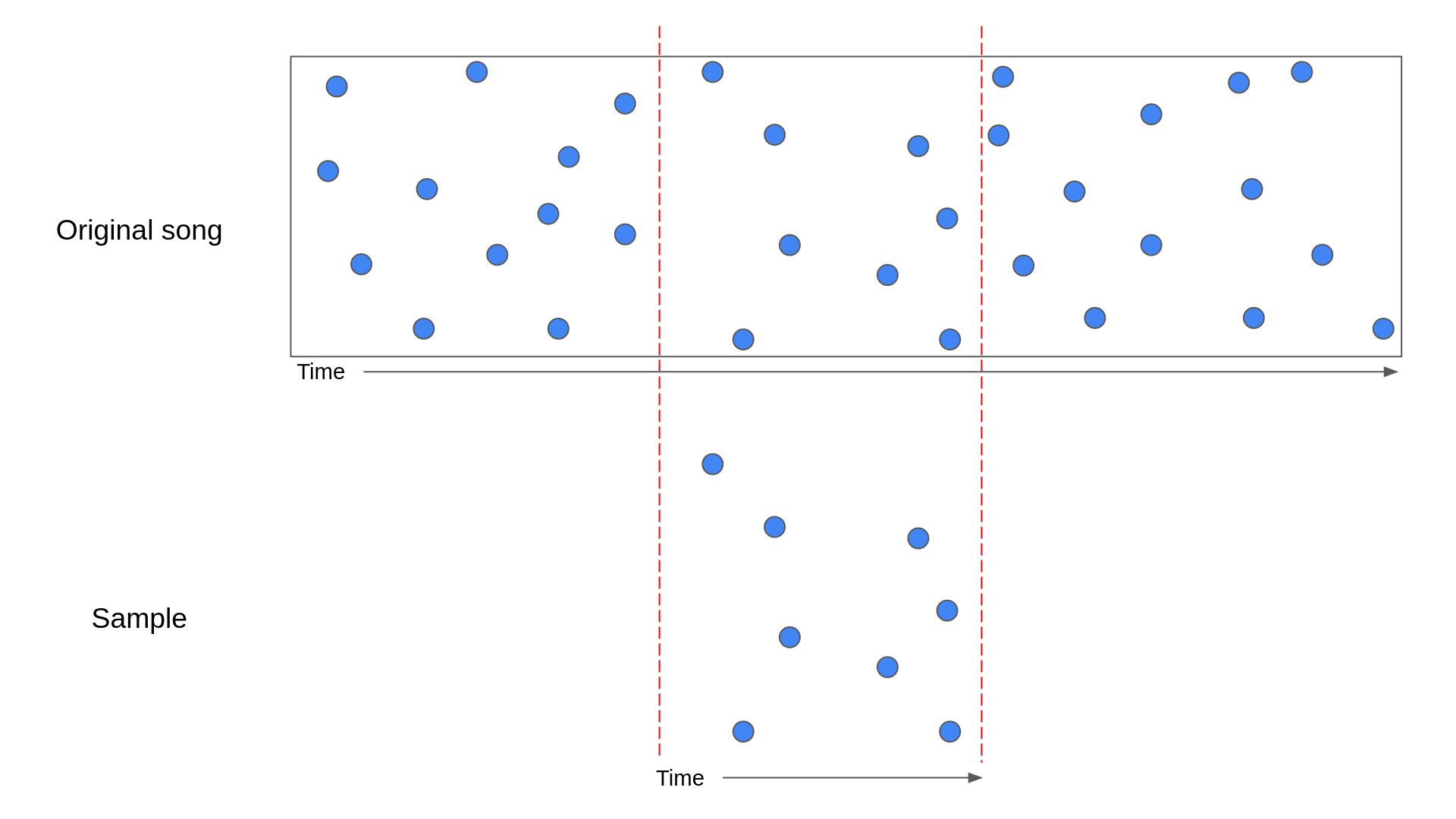
In the above diagram, a sample has been lined up with the section of the original song that it came from. The blue points represent the anchor points of the hashes.
While the above diagram shows the perfect scenario, there is a chance that the matching hashes from the database don't line up perfectly. For example, noise could have introduced peaks in the sample that resemble peaks at a different point in the song. This can lead to the following scenario:
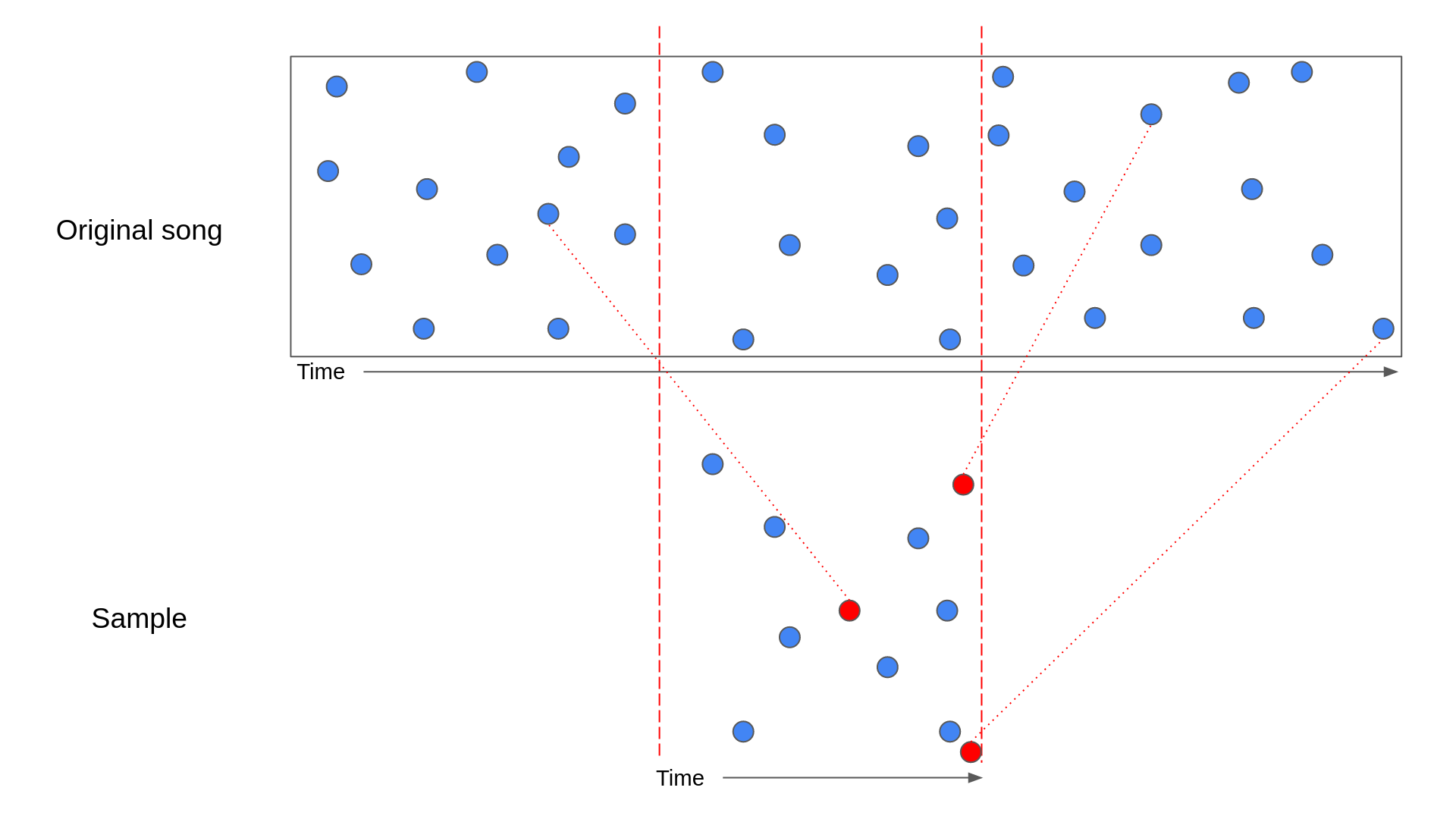
In the above diagram, the red circles represent hashes that match to points in the song outside the section the sample came from. In this situation, it's harder to see that the sample is a perfect match for the song.
What's worse, sometimes hashes can match to the wrong song! This is where checking that the hashes line up comes in.
To explain how we can check whether the hashes line up in code, let's look at an example. Let's imagine that we've got a list of matching hashes from the database and grouped them by track. For a given track, we can then check the time that the hash occurs in the original track against the time that the hash occurs in the sample.
| Sample time | Track time | Track time - Sample time |
|---|---|---|
| 3 | 13 | 10 |
| 4 | 14 | 10 |
| 7 | 20 | 13 |
| 5 | 15 | 10 |
| 6 | 12 | 6 |
| 1 | 11 | 10 |
In the above table, you can see that all the matches with a Track time - Sample time of 10 have been highlighted. These are the true matches, while the other two rows are false matches. To see this is the case, let's look at a similar diagram to the ones we saw before:
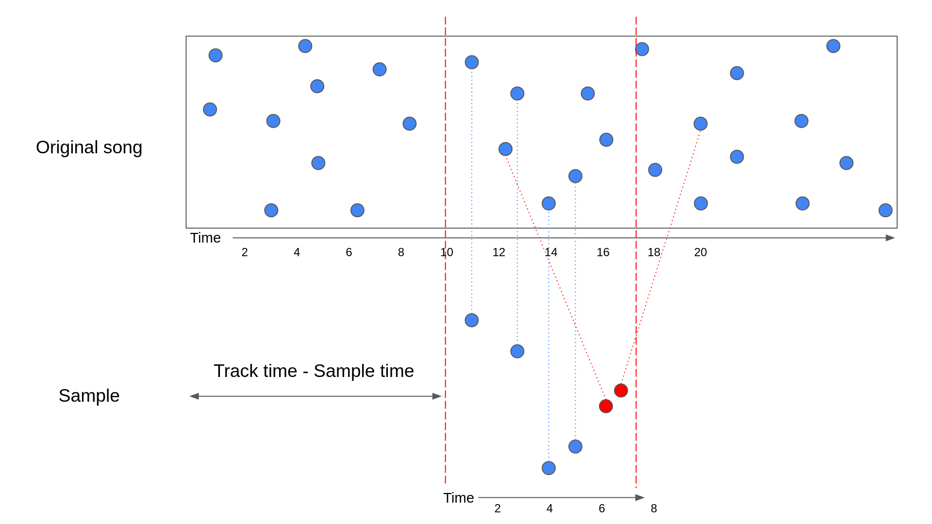
The above diagram contains the same hashes from the previous table. As you can see, the true matches have a Track time - Sample time that is equal to how far into the track time that the sample starts.
To see how we turn this into a score for the track, let's make this data into a histogram. A histogram is a fancy name for a bar chart. We're going to plot each Track time - Sample time against the number of times it occurs:
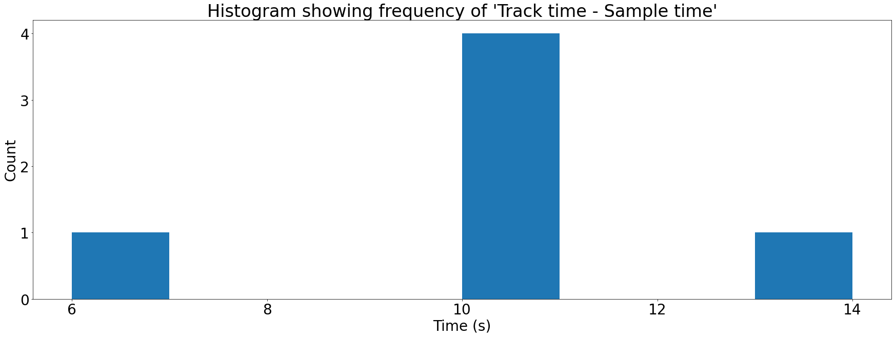
Each bar in the histogram above is referred to as a bin. To score a song on how good a match it is for an audio sample, we just need to take the largest bin. Songs that aren't good matches will have low values in all bins, whereas a song that's a good match will have a large spike in one of the bins.
This way we can compare a sample to all the songs with matching hashes in our database and score each of them. The song with the highest score is likely to be the correct result.
You might wonder why we don't just go for the song that matches the largest number of hashes as it would be much simpler to implement. The problem with this approach is that not all songs are the same length. Longer songs are likely to get more matches than shorter songs and when some Spotify tracks are over 4 hours long this can really bias your results!
Conclusion#
Well done for making it this far, that was a long journey! Over the course of this article, you've learned how Shazam extracts fingerprints from audio, and how it matches these fingerprints to those that it has already registered in its database.
To summarise, Shazam does the following to register a song:
- Calculates a spectrogram of a song
- Extracts peaks from that spectrogram
- Pairs those peaks up into hashes
- Stores the collection of hashes for a song as a fingerprint
Shazam does the following to recognise an audio sample:
- Calculates a fingerprint of the audio sample
- Finds the hashes that match that fingerprint in the database
- For each potential song match:
- Calculate Track time - Sample time for each matching hash
- Group those values into a histogram
- Take the largest bin in this histogram as the score for the song
- Return the song with the highest score
Enter abracadabra#
I learned everything written here over the process of writing abracadabra, my implementation of this paper.
If you are interested in seeing what this might look like in code, please take a look! Everything is open source and I've done my best to document the project. abracadabra can also be used as a library in other projects, so please feel free to re-mix and build something cool. If you do use it, I'd love to hear about it.
Further reading#
If you want to find out more about anything mentioned in this article, take a look below. I've also scattered some helpful links throughout the page.
- abracadabra docs
- dejavu is another implementation of a song recogniser in Python. The author wrote a wonderful explanation on how it works.
- Computer Vision for Music Identification is another approach to song recognition that is similar to how dejavu works.
- An algorithm that takes a slightly different approach is Chromaprint.
- Musicbrainz is an open-source encyclopedia of music information. This page explains how they fingerprint audio.
- Playing with Shazam fingerprints is an article from 2009 about the author's experience implementing the Shazam algorithm.
- Alignment of videos of same event using audio fingerprinting is an example of a use case for this algorithm that goes beyond music.